After students have built, manipulated and discussed the model of the horizontal spring, there are several other models the instructor can choose from to extend the concept. The idea is to have the students recognize that certain key components of the model stay the same and the feedback loop is always present and connected to the same icons. This is what produces the oscillating motion.  In addition, in all these models, the restoring force has a linear dependence on the displacement away from equilibrium, the velocity and acceleration vectors are never pointed in the same direction and the force is constantly changing.

The Vertical Spring

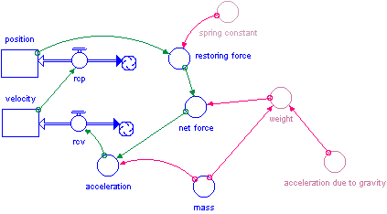
The easiest model to build after the horizontal spring is that of the vertical spring. It can be deceiving. If the only purpose is to show oscillating motion, then very few changes are needed.

There are only three additions to the model: net force, weight and acceleration due to gravity. Net force is equal to the sum of weight and the restoring force. The initial position is set to zero. The model will oscillate with the correct period. This is equivalent to the physical case of hanging a weight on a spring and immediately releasing it. The only drawback to this approach is that the position oscillates between a negative number and zero. Zero being the rest length of the spring before the mass was added. This is not a major flaw, but it could confuse those students who will be asked to perform Hooke’s law calculations in the future. In addition, if energy calculations are added to the model, it can give unsettling results, such as negative gravitational potential energy.

It is not particularly hard to adjust the model for oscillation around zero. One additional term is added which calculates the initial displacement from rest length (weight/spring constant).This resets the zero point to the rest length with the mass hanging on the spring.

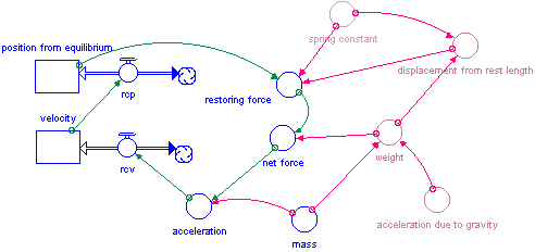
Of course, for the vertical spring, the period is still equal to 2*p* the square root of (m/k). This relationship could be used as one check of the validity of the model.

Hydrometer

The restoring force for a floating object is the buoyant force which is equal to -g*r*A*y, where g is the acceleration due to gravity, r is the density of the liquid,A is the cross sectional area and y is the distance above or below the normal floating layer. There is the additional force of weight acting on the mass. The period is proportional to 2* p * the square root of (m/(g*r*A)).

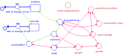
Under Time Specs, the model should run for 3 sec with a DT of 0.05 and Runge-Kutta-4 as the integration method.This model is very close conceptually to the vertical spring and makes a nice extension from that system.

Vibrating Bar

A bar attached at one end, with the other end free to oscillate is another example of a vibrating mechanical system. This system makes an excellent simple physical model of the tuning fork. Students will be able to see the vibrations and can adjust the amplitude in a physical laboratory, neither of which is easily done with a tuning fork.

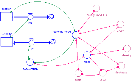
The restoring force of an oscillating metal bar is:

The YM (Young’s Modulus) for aluminum is 7x10¹⁰ N/m².Thickness is measured in the direction of oscillation in m. Width is measured perpendicular to the direction of oscillation in m. Length is measured from oscillating end to clamped end of the bar. Under TimeSpecs, the model should run for 0.06 sec with a DT of 1E-6 and an integration method of Runge-Kutta 4.

The period of the vibrating bar is 2 * p* the square root of ((density * length⁴)/(12.4 * Y * K²)) where K is the radius of gyration and is equal to the thickness/ sqrt(12).

The Tuning Fork

This model is identical to that of the vibrating bar. The only difference is in the choice of physical parameters. Students will need to measure the dimensions of the tuning fork. The length of the tine from the bend up is the length that is entered, but students might be allowed to discover this. They should also determine the density of a tuning fork using water displacement. In addition, tuning forks are usually made of alloys, so students should start with the Young’s modulus for aluminum and adjust this value until the model gives the right frequency. The best use of this model is to put an entire octave of tuning forks in using SensiSpecs and compare the graphs at the same time. It is easy to see the full and half steps of the musical scale.

The restoring force of a struck tuning fork is:

The YM (Young’s Modulus) for aluminum is 7x10¹⁰ N/m². Thickness is measured in the direction of oscillation in m. Width is measured perpendicular to the direction of oscillation in m. Length is measured from top to bottom of tine not the entire length of the fork. Under TimeSpecs, the model should run for 0.005 sec with a DT of 1E-6 and an integration method of Runge-Kutta 4. The formula for the period of the tuning fork is the same as that of the vibrating bar.

Marble in a Bowl

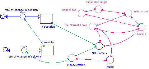
A nice introductory model to the pendulum, is that of a marble rolling back and forth in a bowl. The restoring force comes from the Normal force acting on the marble. However the direction of the Normal force changes as the marble oscillates. The motion can be modeled if you find the x-component of the Normal force. Hence the restoring force will be equivalent to the Normal force * sin(q). Where q is the angle between the extension of the normal force and a radius of the circle that goes through the bottom of the bowl. Furthermore sin(q) equals opposite/hypotenuse which is equivalent to x-position/ radius of the bowl. Under TimeSpecs, the model should run for 6 sec with a DT of 0.1 and an integration method of Runge-Kutta 4. The period = 2 * p * the square root of (r/g) where r is the radius of the bowl and g is the acceleration due to gravity.

Pendulum

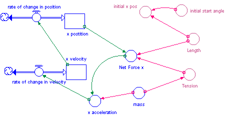
The model for the pendulum can be approached in one of two ways. As an analogy to the marble in the bowl, a model can be built which only concerns itself with the x-component of the force. The x-component of the force is the restoring force. The y-component is not a restoring force and does not affect the period. Treating the model this way allows the students to stay in the Cartesian coordinate system and makes the model very analogous to the marble in the bowl.

The restoring force comes from the tension in the string. However the direction of the tension changes as the pendulum swings. The motion can be modeled if you find the x-component of the Tension. Hence the restoring force will be equivalent to the Tension * sin(q), where q is the angle between the pendulum string and the equilibrium position.Furthermore sin(q) equals opposite/hypotenuse which is equivalent to x-position/length of string. Under TimeSpecs, the model should run for 6 sec with a DT of 0.1 and an integration method of Runge-Kutta 4.

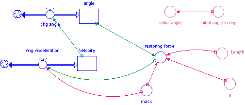
Alternatively, the pendulum can be modeled by using angle instead of position, as well as angular velocity and acceleration. Students do not need to be knowledgeable about polar coordinates, since they are still working in one plane. In addition, this model uses the variables which they will be measuring in lab – angle and length. There is one more concern when using this approach. Most textbooks state that the period is independent of the angle. This is true only for small angles. To be accurate, the restoring force is proportional to sin(q), specifically F = -mgsin(q)/l. The instructor should try to guide the students through the model structure to insure they understand that this is NOT the function producing the oscillating motion. Under TimeSpecs, the model should run for 5 sec with a DT of 0.05 and an integration method of Runge-Kutta 4.

The period of the pendulum is equal to 2 * p * the square root of (l/g).

An applet of the pendulum model shows some of the possible graphs.